Activation Functions

So why do we need Activation functions in our neural networks?

The basic idea of how a neural network learns is - We have some input data that we feed it into the network and then we perform a series of linear operations layer by layer and derive an output. In a simple case for a particular layer is that we multiply the input by the weights, add a bias and apply an activation function and pass the output to the next layer. We keep repeating the process until we reach the last layer. The final value is our output. We then compute the error between the “calculated output” and the “true output” and then calculate the partial derivatives of this error with respect to the parameters in each layer going backwards and keep updating the parameters accordingly!

Neural networks are said to be universal function approximators. The main underlying goal of a neural network is to learn complex non-linear functions. If we do not apply any non-linearity in our multi-layer neural network, we are simply trying to seperate the classes using a linear hyperplane. As we know, in the real-world nothing is linear!

Also, imagine we perform simple linear operation as described above, namely; multiply the input by weights, add a bias and sum them across all the inputs arriving to the neuron. It is likely that in certain situations, the output derived above, takes a large value. When, this output is fed into the further layers, they can be transformed to even larger values, making things computationally uncontrollable. This is where the activation functions play a major role i.e. squashing a real-number to a fix interval (e.g. between -1 and 1).

Let us see different types of activation functions and how they compare against each other:

Sigmoid:

The sigmoid activation function has the mathematical form sig(z) = 1/ (1 + e^-z). As we can see, it basically takes a real valued number as the input and squashes it between 0 and 1. It is often termed as a squashing function as well. It aims to introduce non-linearity in the input space. The non-linearity is where we get the wiggle and the network learns to capture complicated relationships. As we can see from the above mathematical representation, a large negative number passed through the sigmoid function becomes 0 and a large positive number becomes 1. Due to this property, sigmoid function often has a really nice interpretation associated with it as the firing rate of the neuron; from not firing at all (0) to fully-saturated firing at an assumed maximum frequency (1). However, sigmoid activation functions have become less popular over the period of time due to the following two major drawbacks:

• Killing gradients: Sigmoid neurons get saturated on the boundaries and hence the local gradients at these regions is almost zero. To give you a more intuitive example to understand this, consider the inputs to the sigmoid function to be +15 and -15. The derivative of sigmoid function is sig(z) * (1 - sig(z)). As mentioned above, the large positive values are squashed near 1 and large negative values are squashed near 0. Hence, effectively making the local gradient to near 0. As a result, during backpropagation, this gradient gets multiplied to the gradient of this neurons’ output for the final objective function, hence it will effectively “kill” the gradient and no signal will flow through the neuron to its weights. Also, we have to pay attention to initializing the weights of sigmoid neurons to avoid saturation, because, if the initial weights are too large, then most neurons will get saturated and hence the network will hardly learn.

• Non zero-centered outputs: The output is always between 0 and 1, that means that the output after applying sigmoid is always positive hence, during gradient-descent, the gradient on the weights during backpropagation will always be either positive or negative depending on the output of the neuron. As a result, the gradient updates go too far in different directions which makes optimization harder.

The python implementation looks something similar to:

import numpy as np

def sigmoid(z):
	return 1 / (1 + np.exp(-z))

Tanh:

The tanh or hyperbolic tangent activation function has the mathematical form tanh(z) = (e^z - e^-z) / (e^z + e^-z). It is basically a shifted sigmoid neuron. It basically takes a real valued number and squashes it between -1 and +1. Similar to sigmoid neuron, it saturates at large positive and negative values. However, its output is always zero-centered which helps since the neurons in the later layers of the network would be receiving inputs that are zero-centered. Hence, in practice, tanh activation functions are preffered in hidden layers over sigmoid.

import numpy as np

def tanh(z):
	return np.tanh(z)

ReLU:

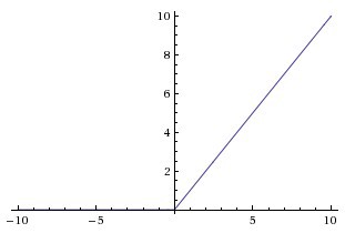
The ReLU or Rectified Linear Unit is represented as ReLU(z) = max(0, z). It basically thresholds the inputs at zero, i.e. all negative values in the input to the ReLU neuron are set to zero. Fairly recently, it has become popular as it was found that it greatly accelerates the convergence of stochastic gradient descent as compared to Sigmoid or Tanh activation functions. Just to give an intuition, the gradient is either 0 or 1 depending on the sign of the input. Let us discuss some of the advantages of ReLU:

• Sparsity of Activations: As we studied above, ReLU and Tanh activation functions would almost always get fired in the neural network, resulting in the almost all the activations getting processed in calculating the final output of the network. Now surely this is a good thing but only if our network is small or we had unlimited computational power. Imagine we have a very deep neural network with a lot of neurons, we would ideally want only a section of neurons to fire and contribute to the final output of the network and hence, we want a section of the neurons in the network to be passive. ReLU gives us this benefit. Hence, due to the characteristics of ReLU, there is a possibility that 50% of neurons to give 0 activations and thus leading to fewer neurons to fire as a result of which the network becomes lighter and we can compute the output faster.

However, it has a drawback in terms of a problem called as dying neurons.

• Dead Neurons: ReLU units can be fragile during training and can “die”. That is, if the units are not activated initially, then during backpropagation zero gradients flow through them. Hence, neurons that “die” will stop responding to the variations in the output error because of which the parameters will never be updated/updated during backpropagation. However, there are concepts such as Leaky ReLU that can be used to overcome this problem. Also, having a proper setting of the learning rate can prevent causing the neurons to be dead.

import numpy as np

def relu(z):
	return z * (z > 0)

Leaky ReLU:

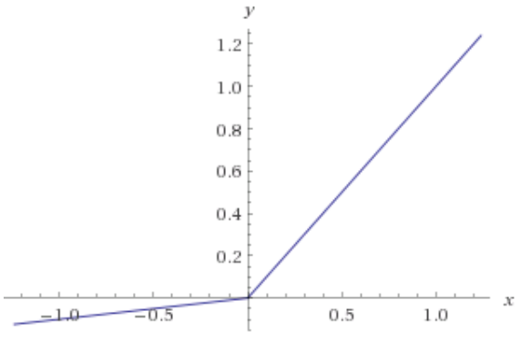
The Leaky ReLU is just an extension of the traditional ReLU function. As we saw that for values less than 0, the gradient is 0 which results in “Dead Neurons” in those regions. To address this problem, Leaky ReLU comes in handy. That is, instead of defining values less than 0 as 0, we instead define negative values as a small linear combination of the input. The small value commonly used is 0.01. It is represented as LeakyReLU(z) = max(0.01 * z, z). The idea of Leaky ReLU can be extended even further by making a small change. Instead of multiplying z with a constant number, we can learn the multiplier and treat it as an additional hyperparameter in our process. This is known as Parametric ReLU. In practice, it is believed that this performs better than Leaky ReLU.

import numpy as np

def leaky_relu(z):
	return np.maximum(0.01 * z, z)

Thank you for reading. In this article I tried to lay down my understanding of some of the most commonly used activation functions, why we use them in the first place and which activation function should one use. Keep chilling and keep innovating!