Gradient Descent - A Beginners Guide

Introduction:

Recently, during my coursework, I have been left in awe of the advancements in the field of science in general. In just about a decade, we have completely revolutionized the way we look at the capabilities of machines, the way we build software and much more. Tasks that seemed impossible just a decade ago have become accessible and effortless. Long story short, we have made the machines think!! Sounds cool, isn’t it? Artificial Intelligence has truly entered the mainstream consciousness. These days every person has heard or read about the two magical words “machine learning” in their day to day life. But how clearly do any of us understand what AI really is? Although, the idea of making machines think and learn sounds fascinating and overwhelming, for aspiring Data Scientists like me to get our heads around; very few understand or know some of the basic concepts that lead to making machines learn.In this blog post, I am simply putting my understanding of one of the most important and the basic technique that is at the core of many machine learning algorithms – Gradient Descent. One of the most critical parts of any machine learning algorithm is optimization. How to make your learning algorithm learn faster? Gradient descent is one of the most powerful optimization algorithm used in machine learning. Many of us have been pretty much familiar with what gradient descent is but when it comes to understanding it, all of us have gone through the process of seeing scary mathematical equations and plots that look something like –

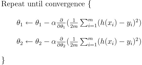
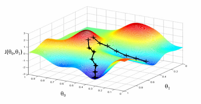
Don’t worry, it is easier than it looks!

As Chris Pine says, “The only thing you sometimes have control over is perspective. You don’t have control over your situation. But you have a choice about how you view it.” Now, let us change our perspective here and see the above plot as something like this-

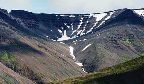
Now, to understand gradient descent, let us imagine the path of the river originating from the top of the mountain. The job of gradient descent is exactly that of what the river aims to achieve; to reach the bottom-most point of the mountain. Now, as we know there is a gravitational force on the earth and hence the river will keep flowing downwards until it reaches the foothill. Here we would be making certain assumptions saying that the mountain will be shaped in such a way that the river will not be stopping at any place and will straightaway arrive at the foothill. In machine learning, this is the ideal case we desire and you can say that we have achieved our “global minima” (in this analogy, it means we have reached the ‘foothill’.). However, in real-life, this is not the case. The way the mountain is, the river may face a lot of pits on its way down and there is a possibility of the water getting trapped in the pits and fail to move downwards. In machine learning terms, this is called “local minima” which is always harmful to any of our learning algorithms. Gradient Descent is prone to arriving at such local minima’s and failing to converge. However, when the mountain terrain is designed in such a particular way i.e. a bowl shape (in machine learning we call such functions as convex functions) then we are guaranteed to arrive at the global minimum (foothill). Now, there are two important points when it comes to gradient descent; initial values and learning rate. To give a general idea about them, we know that depending on where the river initially originates, it will follow a different path to reach the foothill. Also, depending on the speed of the river (learning rate) you might arrive at the foothill in a different manner. These values are important in determining whether you will reach the foothill (global minima) or get trapped in the pits (local minima).

As highlighted above, one of the major reason helping the river flow downwards is the earth’s gravitational force. Sadly in coding/mathematics, we don’t have the leverage of using earth’s gravitational force!! Hence, to overcome this, we need turn to mathematics and need to know two ways to help us move towards the foothill. We do this by calculating 1) the gradient which gives us the direction of the slope and 2) calculating our step-size (i.e. by how many units does the river need to move in a particular direction) Now, let us consider the formula of gradient descent:

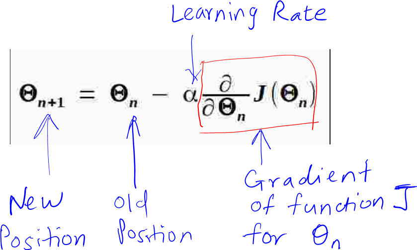
From the above formula, there are two things that we can set on our own; α and the current position of Ɵ. The only thing we need to learn here is, how to calculate the gradient? To calculate the gradient of a function for a point Ɵ, we have to differentiate the function once with respect to Ɵ. Let us understand how to do this with an example:

Consider a function:

f(x, y) = x + y

• We set initial values of x = 2 and y = 6

• The output of the function is 8

• The question here is, how to tweak the values of the inputs to decrease the output?Let us start by differentiating the above function with respect to its inputs; x and y:

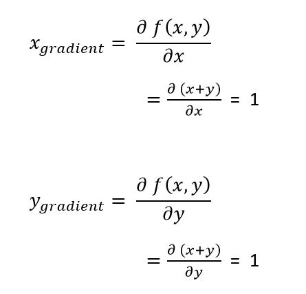
These derivatives can be thought of as the force on each input as we want to pull the output to become as small as possible; forces that tell us how x and y want to change to decrease the output.

Let us see how the update rule works here with our above calculations (let α= 0.001)

This intuitively makes sense! To decrease the output of our function, we need to tweak the inputs x and y with a positive force of magnitude 1. For example, changing the value of x from 2 to 1.999 would give an output of 7.99, which is less than 8 and similarly, by changing the value of y from 6 to 5.999 will give us the output of 7.998, which is less than 8!! The next important characteristic of the gradient descent algorithm is that it is an iterative algorithm! Meaning, we repeat the above steps until convergence.

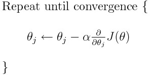
So, if we repeat the above process for 4000 times we will get the value of x = -2 and y = 2.0 leading us to give the output of our function f(x, y) =  0. So we have got the expected values of x and y that cause our function to give the minimum value of 0. This is the intuition behind gradient descent algorithm – one of the “greatest hit” optimization technique that is at the core of most of the machine learning algorithm. I told you, it’s easier than it looks Here, just to make things easy, we have worked with an example that is trivial and low-dimensional. In reality, we will be dealing with non-linear, high-dimensional functions where it is impossible to solve anything by hand analytically. However, the approach works exactly the same there! Does this make sense? Yep? Nope? Although this post is aimed to help beginners get an intuition behind the working of gradient descent, it is by no means a comprehensive overview. Till then, keep chilling and keep innovating!

Lastly, as my friend Gosuddin says “ Jeet k aaenge!”  (Will win)